Sequencing-Based Genetic Study Design with PAWEH
paweh package authors
Source:vignettes/paweh-06-sequencing-study-design.Rmd
paweh-06-sequencing-study-design.RmdOverview
paweh supports prospective analytic power and
minimum-sample-size-necessary (MSSN) calculations for two scientifically
different sequencing designs. The inputs describe a planned experiment;
these functions do not process FASTQ, BAM, or VCF files and do not
perform downstream association testing.
For case-control sequencing designs, sequencing is the common reference:
baseline genotype -> group-specific sequencing call -> Ahn/Chapman–Nam trend NCP -> power or MSSN.
Phenotype misclassification, locus heterogeneity, and conventional genotype misclassification are independent sensitivity scenarios. Each starts from the same biological baseline and uses the same sequencing design; conventional genotype misclassification is applied after the sequencing call.
For affected-child sequencing trios, the pathway is:
latent Mendelian trio state -> raw read-count likelihood -> efficient information -> Kim TDT1-NGS NCP -> power or MSSN.
The case-control calculation therefore propagates uncertainty in called genotypes. TDT1-NGS instead retains raw-read likelihood information and does not hard-call the three genotypes. These are not interchangeable methods.
Two sequencing workflows in paweh
| Feature | Case-control NGS | TDT1-NGS |
|---|---|---|
| Sampling unit | Cases and controls | Complete father-mother-affected-child trios |
| Sequencing information | Called-genotype probabilities | Raw read-count likelihood |
| Association kernel | Ahn/Chapman–Nam trend NCP | Kim efficient-information NCP |
| Public power function | cc_ngs_power() |
tdt_ngs_power() |
| Public MSSN function | cc_ngs_mssn() |
tdt_ngs_mssn() |
| Locus heterogeneity | Available | Ordinary-TDT NCP attenuation sensitivity |
| Phenotype misclassification | Available | Ordinary-TDT NCP attenuation sensitivity |
Both designs use fixed coverage. CC-NGS permits separate case/control depths and errors. TDT1-NGS permits separate father, mother, and child depths with a common directional read-error pair. Neither uses simulation.
Exact published TDT1-NGS replication: the Kim AIS example
Kim (2015) used adolescent idiopathic scoliosis (AIS) to illustrate a
low-coverage trio design. The motivating variant, rs1400180, had a
reported global minor-allele frequency near 0.349; the design
calculation used 0.35. The published assumptions were HWE, symmetric
read error 0.025, genome-wide alpha = 5e-8, a
multiplicative effect reported as OR at least 2, and target power 0.90.
In the TDT1-NGS parameterization this effect is R1 = 2,
with R2 = R1^2.
kim_4x <- tdt_ngs_mssn(
  power = 0.90,
  pd = 0.35,
  R1 = 2,
  coverage = 4,
  seq_error = 0.025,
  alpha = 5e-8,
  verbose = FALSE
)

kim_25x <- tdt_ngs_mssn(
  power = 0.90,
  pd = 0.35,
  R1 = 2,
  coverage = 25,
  seq_error = 0.025,
  alpha = 5e-8,
  verbose = FALSE
)

data.frame(
  coverage = c("4x", "25x"),
  published_trios = c(654, 416),
  paweh_trios = c(kim_4x$MSSN_trios, kim_25x$MSSN_trios)
)
#>   coverage published_trios paweh_trios
#> 1       4x             654         654
#> 2      25x             416         416
Under Kim’s published HWE design with MAF 0.35, symmetric read error
0.025, genome-wide alpha
,
and multiplicative effect R1 = 2, PAWEH exactly reproduces
the reported integer requirements of 654 complete trios at 4x and 416 at
25x for 90% power. This statement applies to this specific published
design and is not a claim about every model in the paper.
Kim’s full Table 3 pairs three target powers with three effect sizes. All six integer results reproduce exactly:
kim_table3 <- data.frame(
  coverage = rep(c(4, 25), times = 3),
  power = rep(c(0.90, 0.70, 0.10), each = 2),
  R1 = rep(c(2.0, 1.8, 1.5), each = 2),
  published_trios = c(654, 416, 716, 456, 733, 466)
)

kim_table3$paweh_trios <- c(
  kim_4x$MSSN_trios,
  kim_25x$MSSN_trios,
  vapply(3:6, function(i) {
    tdt_ngs_mssn(
      power = kim_table3$power[i], pd = 0.35, R1 = kim_table3$R1[i],
      coverage = kim_table3$coverage[i], seq_error = 0.025,
      alpha = 5e-8, verbose = FALSE
    )$MSSN_trios
  }, numeric(1))
)
kim_table3
#>   coverage power  R1 published_trios paweh_trios
#> 1        4   0.9 2.0             654         654
#> 2       25   0.9 2.0             416         416
#> 3        4   0.7 1.8             716         716
#> 4       25   0.7 1.8             456         456
#> 5        4   0.1 1.5             733         733
#> 6       25   0.1 1.5             466         466
TDT1-NGS power and MSSN
For Kim’s one-degree-of-freedom multiplicative model, the NCP is
where is the number of complete trios and is the nuisance-adjusted per-trio information obtained from the raw-read likelihood under the null. The public interface does not require users to manipulate the full information matrix.
tdt_seq_power <- tdt_ngs_power(
  N = 5000,
  pd = 0.325,
  R1 = 1.2,
  coverage = 12,
  seq_error = 0.005,
  alpha = 5e-8,
  verbose = FALSE
)

tdt_seq_mssn <- tdt_ngs_mssn(
  power = 0.80,
  pd = 0.325,
  R1 = 1.2,
  coverage = 12,
  seq_error = 0.005,
  alpha = 5e-8,
  verbose = FALSE
)

data.frame(
  quantity = c("Power at 5,000 trios", "Required trios", "Total individuals"),
  value = c(
    tdt_seq_power$power,
    tdt_seq_mssn$MSSN_trios,
    tdt_seq_mssn$total_individuals
  )
)
#>               quantity        value
#> 1 Power at 5,000 trios 7.072653e-01
#> 2       Required trios 5.507000e+03
#> 3    Total individuals 1.652100e+04
The MSSN calculation first finds the target one-degree-of-freedom NCP and then solves analytically for . It is not an iterative simulation over possible trio counts.
TDT1-NGS can also report phenotype misclassification as a separate
sensitivity scenario. It obtains the ordinary-TDT per-trio coefficient
with and without misclassification and applies
to the sequencing NCP. The bridge fixes
,
,
and
.
Prevalence is used only by this bridge, and pi01 is the
probability that an unaffected individual is misclassified or
ascertained as affected. Kim’s raw-read likelihood, information matrix,
and efficient information are unchanged.
tdt_pheno <- tdt_ngs_power(
  N = 5000, pd = 0.325, R1 = 1.2,
  coverage = 12, seq_error = 0.005,
  pheno_misclass = TRUE, prev = 0.01, pi01 = 0.05,
  alpha = 5e-8, verbose = FALSE
)

data.frame(
  scenario = names(tdt_pheno$scenarios),
  lambda = vapply(tdt_pheno$scenarios, `[[`, numeric(1), "lambda"),
  power = vapply(tdt_pheno$scenarios, `[[`, numeric(1), "power")
)
#>                                                scenario     lambda        power
#> sequencing_only                         sequencing_only 35.9606943 7.072653e-01
#> phenotype_misclassification phenotype_misclassification  0.9419147 3.718473e-06
tdt_pheno$scenarios$phenotype_misclassification$ordinary_tdt_bridge
#> $prev
#> [1] 0.01
#>
#> $pi01
#> [1] 0.05
#>
#> $pd
#> [1] 0.325
#>
#> $R1
#> [1] 1.2
#>
#> $R2
#> [1] 1.44
#>
#> $delta_prime
#> [1] 1
#>
#> $theta1
#> [1] 0.325
#>
#> $gT_noerror
#> [1] 0.233794
#>
#> $gNT_noerror
#> [1] 0.219375
#>
#> $ncp_per_trio_noerror
#> [1] 0.0009175736
#>
#> $gT_pheno
#> [1] 0.2216772
#>
#> $gNT_pheno
#> [1] 0.219375
#>
#> $ncp_per_trio_pheno
#> [1] 2.403391e-05
#>
#> $attenuation_factor
#> [1] 0.02619289
#>
#> $status
#> [1] "estimated"
#>
#> $method
#> [1] "ordinary_TDT_NCP_attenuation_bridge"
#>
#> $raw_read_likelihood_modified
#> [1] FALSE
The phenotype scenario scales the per-trio coefficient before MSSN inversion. It is an ordinary-TDT attenuation bridge, not a phenotype-aware raw-read likelihood, TDTae, or simulation.
Locus heterogeneity is a second independent sensitivity scenario. Its
public parameter is the heterogeneous trio fraction
heter_rate; the linked or homogeneous fraction in the
ordinary TDT equations is
.
The bridge applies
to the same sequencing-only NCP.
tdt_het <- tdt_ngs_power(
  N = 5000, pd = 0.325, R1 = 1.2,
  coverage = 12, seq_error = 0.005,
  locus_het = TRUE, prev = 0.01, heter_rate = 0.25,
  alpha = 5e-8, verbose = FALSE
)
tdt_het$scenarios$heterogeneity$ordinary_tdt_bridge
#> $modifier
#> [1] "locus_heterogeneity"
#>
#> $prev
#> [1] 0.01
#>
#> $heter_rate
#> [1] 0.25
#>
#> $effective_pi
#> [1] 0.75
#>
#> $pd
#> [1] 0.325
#>
#> $R1
#> [1] 1.2
#>
#> $R2
#> [1] 1.44
#>
#> $delta_prime
#> [1] 1
#>
#> $theta1
#> [1] 0.325
#>
#> $gT_noerror
#> [1] 0.233794
#>
#> $gNT_noerror
#> [1] 0.219375
#>
#> $ncp_per_trio_noerror
#> [1] 0.0009175736
#>
#> $gT_heterogeneity
#> [1] 0.2319916
#>
#> $gNT_heterogeneity
#> [1] 0.2211774
#>
#> $ncp_per_trio_heterogeneity
#> [1] 0.0005161352
#>
#> $attenuation_factor
#> [1] 0.5625
#>
#> $status
#> [1] "estimated"
#>
#> $method
#> [1] "ordinary_TDT_NCP_attenuation_bridge"
#>
#> $raw_read_likelihood_modified
#> [1] FALSE
When both modifiers are requested, scenarios contains
sequencing_only, phenotype_misclassification,
and heterogeneity in that order. The two modifier scenarios
each start from sequencing_only; PAWEH does not multiply
their attenuation factors or report a combined modifier result.
coverage remains shorthand for one equal fixed depth.
The optional father_coverage, mother_coverage,
and child_coverage arguments override it independently.
Likewise, seq_error sets the symmetric shorthand
epsilon0 = epsilon1 = seq_error; either directional value
can override its side, and seq_error may be omitted when
both are supplied.
tdt_member_specific <- tdt_ngs_power(
  N = 5000, pd = 0.325, R1 = 1.2,
  father_coverage = 6, mother_coverage = 12, child_coverage = 20,
  epsilon0 = 0.005, epsilon1 = 0.015,
  alpha = 5e-8, verbose = FALSE
)
tdt_member_specific$sequencing
#> $coverage
#> father mother  child
#>      6     12     20
#>
#> $father_coverage
#> [1] 6
#>
#> $mother_coverage
#> [1] 12
#>
#> $child_coverage
#> [1] 20
#>
#> $epsilon0
#> [1] 0.005
#>
#> $epsilon1
#> [1] 0.015
#>
#> $equal_coverage
#> [1] FALSE
#>
#> $symmetric_error
#> [1] FALSE
The directional convention is . Thus a genotype-0 read is alternative with probability , a genotype-2 read is alternative with probability , and a heterozygote has probability . The heterozygote probability is one-half when the errors are symmetric. These settings enter the same raw-read latent-state likelihood; genotypes are not hard-called.
TDT sequencing sensitivity
A small coverage-by-error grid helps identify whether a proposed design is in a steep low-depth region or near a higher-depth plateau.
plot_ngs_power(
  design = "tdt",
  coverage = c(2, 4, 8, 12, 20),
  seq_error = c(0.005, 0.01),
  target_power = 0.80,
  N = 5000, pd = 0.325, R1 = 1.2, alpha = 5e-8
)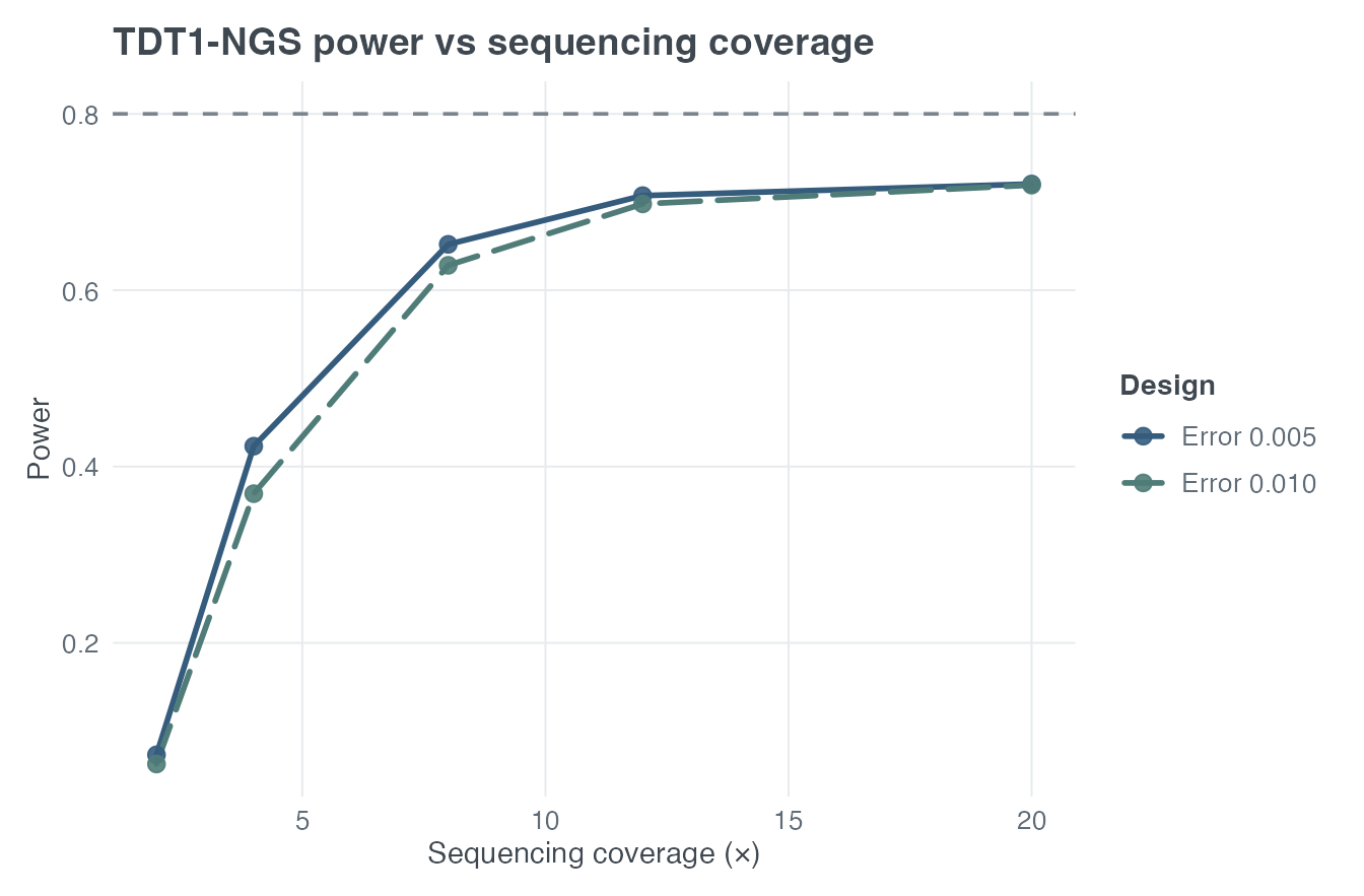
TDT1-NGS power across equal fixed coverage for two symmetric per-read error assumptions.
plot_ngs_mssn(
  design = "tdt",
  coverage = c(2, 4, 8, 12, 20),
  seq_error = c(0.005, 0.01),
  power = 0.80, pd = 0.325, R1 = 1.2, alpha = 5e-8
)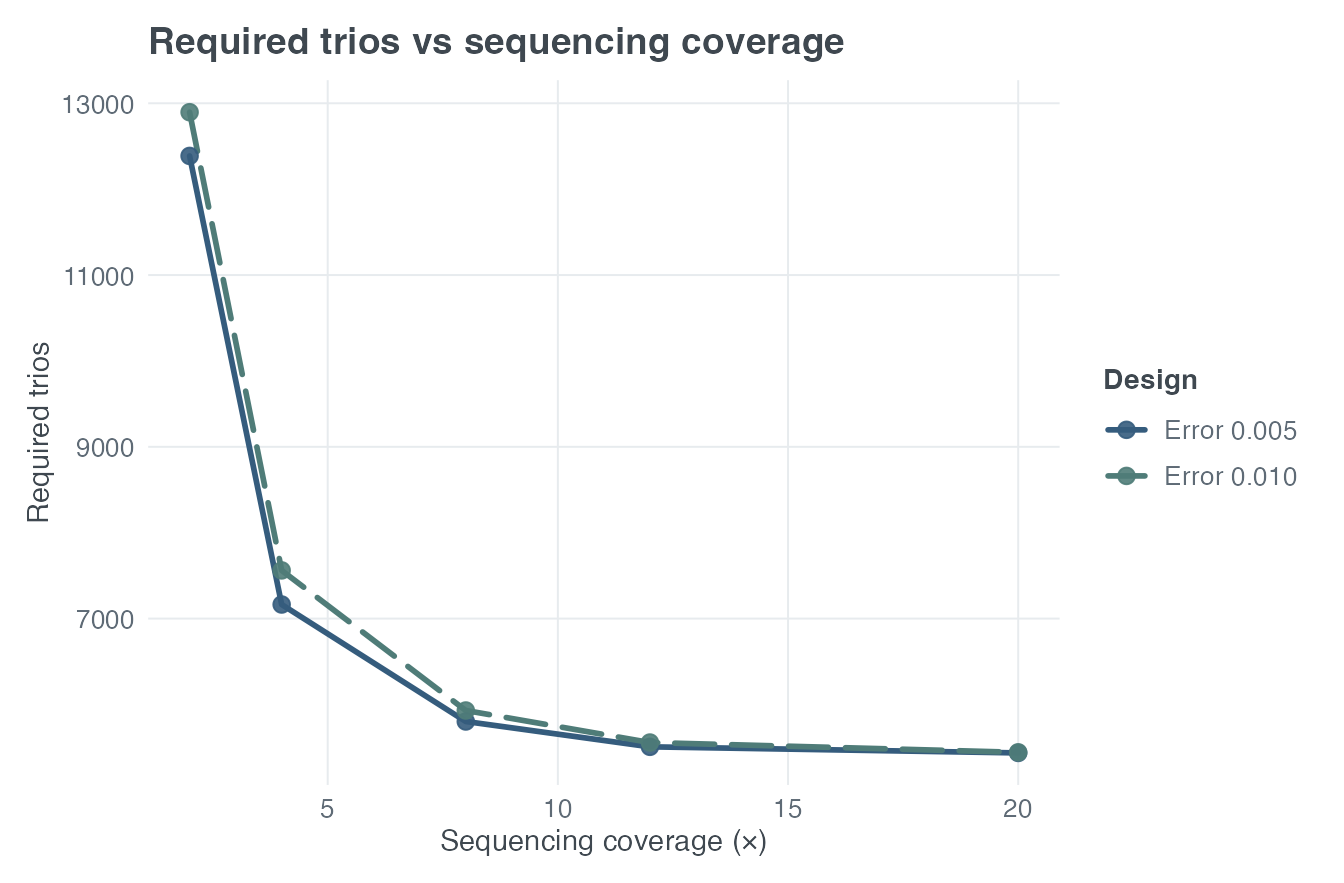
Required complete trios across equal fixed coverage for two symmetric per-read error assumptions.
Low-to-moderate depth gains can be large, whereas gains at higher depth may plateau. The effect of sequencing error remains setting-dependent and should not be assumed negligible. The current fixed-depth TDT1-NGS implementation does not support a design in which any trio member is modeled at exactly 1x coverage under the full nuisance parameterization. This is a specific identifiability boundary of the implemented model, not a claim that 1x sequencing is universally unusable.
Published case-control framework: the Ahn example
Ahn et al. (2007) studied ordinary genotype misclassification, not
sequencing depth. The paper supplies genotype-error probabilities
directly. PAWEH implements Ahn Equation (1), its analytic MSSN
rearrangement, and the published trend scores T001 =
(0,0,1), T011 = (0,1,1), and T012 =
(0,1,2).
The stronger numerical example uses prevalence 0.005, marker and
disease allele frequencies 0.30,
,
and relative risks 2 and 3. The following conditional frequencies were
independently reconstructed from Ahn’s genetic model during package
validation. Adjacent-genotype errors of 5% correspond to the PAWEH
three-parameter matrix with e01 = e02 = 0.05 and
e03 = 0.
ahn_case <- c(0.398125, 0.472500, 0.129375)
ahn_control <- c(0.490461683417085, 0.419736180904523, 0.089802135678392)

ahn_no_error <- cc_power(
  N_case = 1000, alpha = 0.001,
  input_mode = "model_free",
  g1 = ahn_case, g0 = ahn_control,
  k = 1, w = c(0, 1, 2),
  geno_misclass = "none", verbose = FALSE
)

ahn_adjacent_error <- cc_power(
  N_case = 1000, alpha = 0.001,
  input_mode = "model_free",
  g1 = ahn_case, g0 = ahn_control,
  k = 1, w = c(0, 1, 2),
  geno_misclass = "3p", e01 = 0.05, e02 = 0.05, e03 = 0,
  verbose = FALSE
)

data.frame(
  scenario = c("No error", "No error", "5% adjacent error", "5% adjacent error"),
  test = c("T012", "Genotype chi-square", "T012", "Genotype chi-square"),
  published_approximate_power = c(0.88, 0.81, 0.79, 0.70),
  paweh_power = c(
    ahn_no_error$tests$trend$power,
    ahn_no_error$tests$genotypes$power,
    ahn_adjacent_error$tests$trend$power,
    ahn_adjacent_error$tests$genotypes$power
  )
)
#>            scenario                test published_approximate_power paweh_power
#> 1          No error                T012                        0.88   0.8742681
#> 2          No error Genotype chi-square                        0.81   0.8060845
#> 3 5% adjacent error                T012                        0.79   0.7875922
#> 4 5% adjacent error Genotype chi-square                        0.70   0.6992310
This is a Published-method replication, not a CC-NGS sequencing-depth replication. PAWEH implements Ahn’s Equation (1) exactly and closely reproduces the paper’s ordinary genotype-misclassification power example.
The PAWEH CC-NGS sequencing bridge
Ahn takes as an input. PAWEH adds an upstream analytic bridge from sequencing assumptions to those probabilities. For true genotype , alternate-read count , and fixed depth ,
A deterministic maximum-likelihood rule calls genotype . Each transition probability
is obtained by finite summation over all possible read counts. Rows of are true genotypes and columns are called genotypes. This coverage-to-matrix bridge is a PAWEH composition; it was not proposed in the Ahn paper.
ngs_genotype_error_matrix(coverage = 4, seq_error = 0.005)
#>            called_0  called_1     called_2
#> true_0 9.801495e-01 0.0198505 6.250000e-10
#> true_1 6.250000e-02 0.8750000 6.250000e-02
#> true_2 6.250000e-10 0.0198505 9.801495e-01
CC-NGS power and MSSN
The public case-control interfaces construct true case and control genotype probabilities from the disease model, apply the sequencing transition matrix, optionally apply the ordinary PAWEH genotype-misclassification model, and then use the Ahn/Chapman–Nam trend NCP.
cc_seq_power <- cc_ngs_power(
  N_case = 1000,
  alpha = 5e-8,
  prev = 0.05,
  pd = 0.30,
  R2 = 1.8,
  coverage = 4,
  seq_error = 0.005,
  MOI = "M",
  k = 1,
  verbose = FALSE
)

cc_seq_mssn <- cc_ngs_mssn(
  power = 0.80,
  alpha = 5e-8,
  prev = 0.05,
  pd = 0.30,
  R2 = 1.8,
  coverage = 4,
  seq_error = 0.005,
  MOI = "M",
  k = 1,
  verbose = FALSE
)

data.frame(
  quantity = c(
    "Power at 1,000 cases", "Required cases", "Required controls", "Total MSSN"
  ),
  value = c(
    cc_seq_power$power,
    cc_seq_mssn$MSSN_case,
    cc_seq_mssn$MSSN_ctrl,
    cc_seq_mssn$MSSN_total
  )
)
#>               quantity        value
#> 1 Power at 1,000 cases    0.1197042
#> 2       Required cases 2168.0000000
#> 3    Required controls 2168.0000000
#> 4           Total MSSN 4336.0000000
Sequencing uncertainty is upstream of the published trend NCP. The MSSN calculation remains analytic after inversion of the target NCP.
Separate case/control sequencing
For both cc_ngs_power() and cc_ngs_mssn(),
coverage and seq_error remain common
shorthand. case_coverage and ctrl_coverage
independently override coverage;
case_seq_error and ctrl_seq_error
independently override seq_error. A common parameter may be
omitted when both corresponding overrides are supplied. Explicit invalid
overrides, including NULL, are rejected. Only effective
parameters are validated.
cc_differential <- cc_ngs_power(
  N_case = 1000, alpha = 0.05, prev = 0.05, pd = 0.30, R2 = 1.8,
  coverage = 10, seq_error = 0.01,
  case_coverage = 4, case_seq_error = 0.04,
  locus_het = TRUE, pi = 0.75, verbose = FALSE
)
cc_differential$sequencing
#> $case_coverage
#> [1] 4
#>
#> $ctrl_coverage
#> [1] 10
#>
#> $case_seq_error
#> [1] 0.04
#>
#> $ctrl_seq_error
#> [1] 0.01
#>
#> $case_transition_matrix
#>          called_0  called_1   called_2
#> true_0 0.84934656 0.1506509 0.00000256
#> true_1 0.06250000 0.8750000 0.06250000
#> true_2 0.00000256 0.1506509 0.84934656
#>
#> $ctrl_transition_matrix
#>            called_0  called_1     called_2
#> true_0 9.957338e-01 0.0042662 9.910000e-18
#> true_1 1.074219e-02 0.9785156 1.074219e-02
#> true_2 9.910000e-18 0.0042662 9.957338e-01
CC-NGS also accepts the ordinary case-control phenotype-error
parameters: pheno_misclass, theta, and
phi. Here theta is the probability that a
truly affected individual is classified as a control, and
phi is the probability that a truly unaffected individual
is classified as a case. The transformation uses disease prevalence
exactly as cc_power() and cc_mssn() do.
cc_pheno_differential <- cc_ngs_power(
  N_case = 1000, alpha = 0.05, prev = 0.05, pd = 0.30, R2 = 1.8,
  coverage = 10, seq_error = 0.01,
  case_coverage = 4, case_seq_error = 0.04,
  locus_het = TRUE, pi = 0.75,
  pheno_misclass = TRUE, theta = 0.02, phi = 0.01,
  verbose = FALSE
)
cc_pheno_differential$errors$phenotype_misclass
#> $enabled
#> [1] FALSE
#>
#> $theta
#> [1] 0.02
#>
#> $phi
#> [1] 0.01
#>
#> $g_case_before_pheno_misclass
#> [1] 0.4031299 0.4635904 0.1332797
#>
#> $g_ctrl_before_pheno_misclass
#> [1] 0.49457211 0.41770577 0.08772212
#>
#> $g_case_after_pheno_misclass
#> [1] 0.4031299 0.4635904 0.1332797
#>
#> $g_ctrl_after_pheno_misclass
#> [1] 0.49457211 0.41770577 0.08772212
#>
#> $case_denom
#> [1] NA
#>
#> $ctrl_denom
#> [1] NA
The same interfaces support ordinary case-control "1p",
"2p", "3p", and "diff3p" genotype
misclassification after sequencing. Sequencing models read and
genotype-call uncertainty; geno_misclass then models error
in those called genotypes. Both stages may be active, and each may
differ between cases and controls.
cc_all_errors <- cc_ngs_power(
  N_case = 1000, alpha = 0.05, prev = 0.05, pd = 0.30, R2 = 1.8,
  case_coverage = 4, ctrl_coverage = 10,
  case_seq_error = 0.04, ctrl_seq_error = 0.01,
  locus_het = TRUE, pi = 0.75,
  pheno_misclass = TRUE, theta = 0.02, phi = 0.01,
  geno_misclass = "diff3p",
  case_e01 = 0.03, case_e02 = 0.01, case_e03 = 0.004,
  ctrl_e01 = 0.01, ctrl_e02 = 0.005, ctrl_e03 = 0.002,
  verbose = FALSE
)
names(cc_all_errors$scenarios)
#> [1] "sequencing_only"             "phenotype_misclassification"
#> [3] "heterogeneity"               "genotype_misclassification"
cc_all_errors$scenarios$genotype_misclassification$errors$genotype_misclass
#> $enabled
#> [1] TRUE
#>
#> $model
#> [1] "diff3p_homhet_homhom"
#>
#> $diff_source
#> [1] "explicit"
#>
#> $diff_multiplier
#> [1] 1
#>
#> $case_params
#>   e01   e02   e03
#> 0.030 0.010 0.004
#>
#> $ctrl_params
#>   e01   e02   e03
#> 0.010 0.005 0.002
#>
#> $M_case
#>       [,1] [,2]  [,3]
#> [1,] 0.966 0.03 0.004
#> [2,] 0.010 0.98 0.010
#> [3,] 0.004 0.03 0.966
#>
#> $M_ctrl
#>       [,1] [,2]  [,3]
#> [1,] 0.988 0.01 0.002
#> [2,] 0.005 0.99 0.005
#> [3,] 0.002 0.01 0.988
CC-NGS always reports sequencing_only. Requested
phenotype and heterogeneity scenarios transform the biological baseline
before group-specific sequencing. The requested
genotype-misclassification scenario sequences the unmodified baseline
first and applies conventional genotype error to the called genotypes.
Multiple modifiers request multiple independent results rather than a
combined error path. The sequencing matrices give
t(M_seq_case) %*% g_case_preseq and
t(M_seq_ctrl) %*% g_ctrl_preseq. In the genotype scenario,
the genotype-error matrices then transform those calls. All matrices
have current-genotype rows and observed-genotype columns; equivalently,
each group’s genotype scenario uses M_seq %*% M_geno.
The sequencing list records all four effective
parameters and both matrices. Legacy coverage and
seq_error fields retain common inputs (or NULL
if omitted); transition_matrix retains the case matrix,
shared by both groups when settings are equal. Use the explicit matrices
for differential designs. The freqs list exposes
post-heterogeneity and pre-sequencing frequencies, and the
errors$phenotype_misclass list records the phenotype
transformation and its observed-group denominators. Post-sequencing and
final frequencies are available in freqs, while
errors$genotype_misclass records the selected model,
parameters, and case/control matrices.
Different sequencing or genotype-error mechanisms can create observed
differences even under a biological null. Power and MSSN are nominal
asymptotic results using the existing chi-square critical value; neither
the null distribution nor Type I error is independently recalibrated for
differential observation. In particular, pi = 0 need not
remove the observed contrast. Plot extensions are deferred; the plotting
examples below use common sequencing settings.
Why zero per-read error is not perfect at finite depth
Setting seq_error = 0 eliminates incorrect base reads,
but it does not make finite-depth heterozygote calls perfect. For a true
heterozygote,
At low , every observed read can come from the same allele. Such an observation can be more likely under a homozygous genotype, creating call uncertainty even with no per-read sequencing error. This probability decreases with depth but is nonzero at every finite depth.
list(
  coverage_2 = ngs_genotype_error_matrix(2, 0),
  coverage_10 = ngs_genotype_error_matrix(10, 0)
)
#> $coverage_2
#>        called_0 called_1 called_2
#> true_0     1.00      0.0     0.00
#> true_1     0.25      0.5     0.25
#> true_2     0.00      0.0     1.00
#>
#> $coverage_10
#>            called_0  called_1     called_2
#> true_0 1.0000000000 0.0000000 0.0000000000
#> true_1 0.0009765625 0.9980469 0.0009765625
#> true_2 0.0000000000 0.0000000 1.0000000000
CC sequencing sensitivity
plot_ngs_power(
  design = "cc",
  coverage = c(2, 4, 8, 12, 20),
  seq_error = c(0.005, 0.01),
  target_power = 0.80,
  N_case = 1000, alpha = 5e-8,
  prev = 0.05, pd = 0.30, R2 = 1.8, MOI = "M", k = 1
)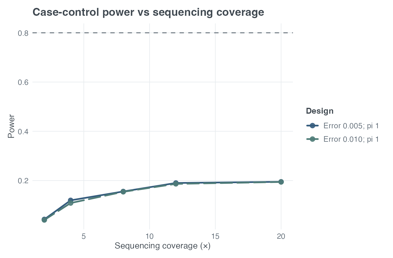
Case-control sequencing trend power across equal fixed coverage for two symmetric per-read error assumptions.
plot_ngs_mssn(
  design = "cc",
  coverage = c(2, 4, 8, 12, 20),
  seq_error = c(0.005, 0.01),
  power = 0.80, alpha = 5e-8,
  prev = 0.05, pd = 0.30, R2 = 1.8, MOI = "M", k = 1
)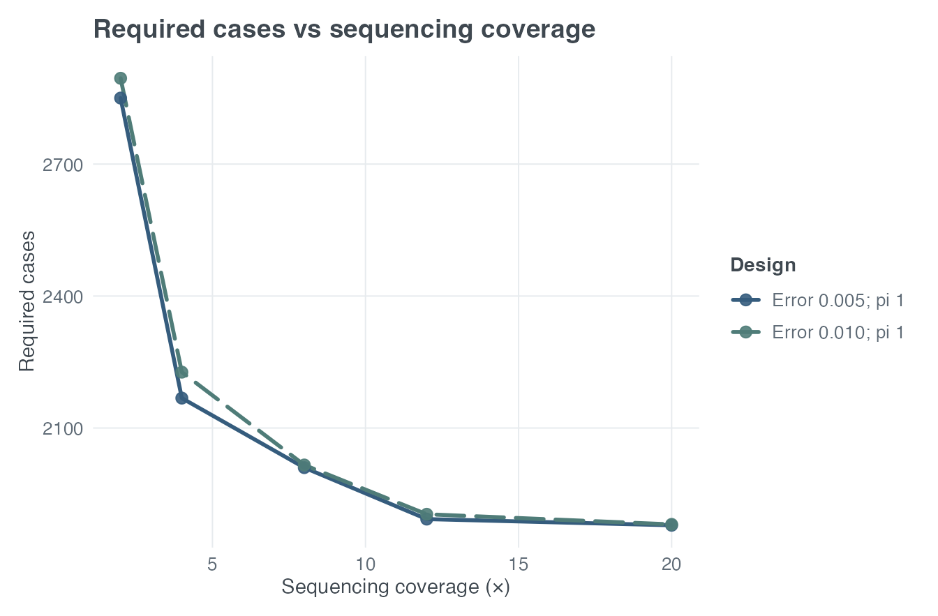
Required case sample size across equal fixed coverage for two symmetric per-read error assumptions.
These are deterministic scenario curves, not uncertainty bands. A robust design should be examined over scientifically plausible depth and error values rather than only at a single optimistic point.
CC locus heterogeneity
Case-control sequencing designs can dilute the associated-case distribution with the control distribution:
Here pi = 1 retains the full locus-associated case
distribution and pi = 0 removes the locus-specific
contrast. The master switch is strict: when
locus_het = FALSE, pi must remain 1.
cc_heterogeneous <- cc_ngs_power(
  N_case = 1000, alpha = 0.05,
  prev = 0.05, pd = 0.30, R2 = 1.8,
  coverage = 4, seq_error = 0.005,
  MOI = "M", k = 1,
  locus_het = TRUE, pi = 0.75,
  verbose = FALSE
)

data.frame(
  pi = cc_heterogeneous$locus_het$pi,
  lambda = cc_heterogeneous$lambda,
  power = cc_heterogeneous$power
)
#>     pi   lambda     power
#> 1 0.75 10.41674 0.8975178
The exact pi = 0 boundary
With equal sequencing mechanisms and
locus_het = TRUE, pi = 0, case and control called genotype
distributions are identical. Therefore the NCP is zero and power equals
alpha. If requested power exceeds alpha, no
finite sample size exists.
The plotting-data interface preserves this scientific boundary instead of inventing a very large finite MSSN:
pi_boundary <- plot_ngs_mssn(
  design = "cc",
  coverage = 4,
  seq_error = 0.005,
  return_data = TRUE,
  power = 0.80, alpha = 0.05,
  prev = 0.05, pd = 0.30, R2 = 1.8, MOI = "M", k = 1,
  locus_het = TRUE, pi = c(1, 0.75, 0.50, 0)
)

pi_boundary[, c("pi", "MSSN_case", "finite_mssn", "status")]
#>     pi MSSN_case finite_mssn         status
#> 1 1.00       430        TRUE         finite
#> 2 0.75       754        TRUE         finite
#> 3 0.50      1671        TRUE         finite
#> 4 0.00        NA       FALSE no finite MSSN
The pi = 0 row remains visible with
MSSN_case = NA, finite_mssn = FALSE, and
status "no finite MSSN".
Fixed-depth assumptions and limitations
CC-NGS assumes fixed coverage within each group; TDT1-NGS allows a separate fixed coverage value for each trio member. They do not yet integrate over a realistic empirical or budget-generated coverage distribution in which a locus may be 0x in some samples, 1x or 2x in others, and 4x or greater elsewhere. Variable/BGE coverage-distribution modeling is deferred.
| Assumption | CC-NGS | TDT1-NGS |
|---|---|---|
| Locus | Single biallelic | Single biallelic |
| Sampling | Cases and controls | Complete affected-child trios |
| Genetic model | M, dominant, or recessive trend scores | Multiplicative |
| Parental HWE/random mating | Not applicable | Assumed by current public design |
| Coverage | Fixed depth per group | Fixed depth per trio member |
| Public read error | Symmetric | Common directional pair |
| Sequencing analysis | Deterministic genotype calls | Raw-read latent-state likelihood |
| Case/control observation error | Common or differential sequencing | Not applicable |
| Locus heterogeneity | Optional canonical mixture | Optional ordinary-TDT NCP attenuation bridge |
| Phenotype misclassification | Optional prevalence-weighted mixture | Optional ordinary-TDT NCP attenuation bridge |
| Genotype misclassification | Optional 1p, 2p, 3p, or differential 3p | Not implemented |
| Simulation | None | None |
Deferred capabilities include variable/BGE coverage, simulation validation, cost-depth optimization, TDT genotype misclassification, and a sequencing Shiny module. The existing dashboard covers the non-sequencing study-design modules.
A practical design workflow
- Choose an unrelated case-control or affected-child trio design.
- Specify allele-frequency and effect assumptions from defensible prior data.
- Choose candidate fixed coverage and per-read error scenarios.
- Calculate power at the available sample size.
- Calculate MSSN for the target power.
- Plot coverage and sequencing-error sensitivity.
- For case-control designs, stress-test plausible locus heterogeneity.
- Report the model, fixed-depth assumption, sampling unit, error assumption, and sensitivity range with the design recommendation.
References
Ahn K, Haynes C, Kim W, St Fleur R, Gordon D, Finch SJ. The effects of SNP genotyping errors on the power of the Cochran-Armitage linear trend test for case/control association studies. Annals of Human Genetics. 2007;71(2):249–261. https://doi.org/10.1111/j.1469-1809.2006.00318.x.
Chapman DG, Nam JM. Asymptotic power of chi square tests for linear trends in proportions. Biometrics. 1968;24(2):315–327. https://doi.org/10.2307/2528035.
Gordon D, Finch SJ, Kim W. Heterogeneity in Statistical Genetics: How to Assess, Address, and Account for Mixtures in Association Studies. Springer; 2020. https://doi.org/10.1007/978-3-030-61121-7.
Kim W. Transmission disequilibrium tests based on read counts for low-coverage next-generation sequence data. Human Heredity. 2015;80(1):36–49. https://doi.org/10.1159/000434645.
Session information
sessionInfo()
#> R version 4.6.1 (2026-06-24)
#> Platform: aarch64-apple-darwin23
#> Running under: macOS Tahoe 26.6.2
#>
#> Matrix products: default
#> BLAS:   /Library/Frameworks/R.framework/Versions/4.6/Resources/lib/libRblas.0.dylib
#> LAPACK: /Library/Frameworks/R.framework/Versions/4.6/Resources/lib/libRlapack.dylib;  LAPACK version 3.12.1
#>
#> locale:
#> [1] C.UTF-8/C.UTF-8/C.UTF-8/C/C.UTF-8/C.UTF-8
#>
#> time zone: America/New_York
#> tzcode source: internal
#>
#> attached base packages:
#> [1] stats     graphics  grDevices utils     datasets  methods   base
#>
#> other attached packages:
#> [1] paweh_0.99.0     BiocStyle_2.40.0
#>
#> loaded via a namespace (and not attached):
#>  [1] gtable_0.3.6        jsonlite_2.0.0      dplyr_1.2.1
#>  [4] compiler_4.6.1      BiocManager_1.30.27 tidyselect_1.2.1
#>  [7] dichromat_2.0-1     jquerylib_0.1.4     systemfonts_1.3.2
#> [10] scales_1.4.0        textshaping_1.0.5   yaml_2.3.12
#> [13] fastmap_1.2.0       ggplot2_4.0.3       R6_2.6.1
#> [16] labeling_0.4.3      generics_0.1.4      knitr_1.51
#> [19] htmlwidgets_1.6.4   tibble_3.3.1        bookdown_0.47
#> [22] desc_1.4.3          bslib_0.12.0        pillar_1.11.1
#> [25] RColorBrewer_1.1-3  rlang_1.3.0         cachem_1.1.0
#> [28] xfun_0.60           fs_2.1.0            sass_0.4.10
#> [31] S7_0.2.2            otel_0.2.0          cli_3.6.6
#> [34] withr_3.0.3         pkgdown_2.2.1       magrittr_2.0.5
#> [37] digest_0.6.39       grid_4.6.1          mvtnorm_1.4-2
#> [40] lifecycle_1.0.5     vctrs_0.7.3         evaluate_1.0.5
#> [43] glue_1.8.1          farver_2.1.2        ragg_1.5.2
#> [46] rmarkdown_2.31      pkgconfig_2.0.3     tools_4.6.1
#> [49] htmltools_0.5.9