Case-control genetic association study design

From a scientific contrast to a design

A case-control association study asks whether genotype distributions differ between affected and unaffected groups. paweh supports the two-degree-of- freedom genotype chi-square test and a one-degree-of-freedom genotype trend test. The control-to-case ratio k connects the two sample sizes:

$N_{control}=kN_{case}.$

In model-based designs, prevalence, disease-allele frequency, relative risk, and mode of inheritance determine the conditional genotype distributions. In model-free designs, the researcher supplies those distributions directly as g1 (case or affected) and g0 (control or unaffected).

Basic power and inverse design

The unified interfaces are the normal starting point. This model-based example asks for power with 500 cases and an equal number of controls, then solves the inverse problem for 80% power.

basic_cc_power <- cc_power(
  N_case = 500, alpha = 0.05,
  input_mode = "model_based",
  prev = 0.05, pd = 0.30, R2 = 1.8, MOI = "M",
  k = 1, verbose = FALSE
)

basic_cc_mssn <- cc_mssn(
  power = 0.80, alpha = 0.05,
  input_mode = "model_based",
  prev = 0.05, pd = 0.30, R2 = 1.8, MOI = "M",
  k = 1, verbose = FALSE
)

data.frame(
  quantity = c("Genotype-test power", "Required cases", "Required controls", "Required total"),
  value = c(
    basic_cc_power$tests$genotypes$power,
    basic_cc_mssn$tests$genotypes$MSSN_case,
    basic_cc_mssn$tests$genotypes$MSSN_ctrl,
    basic_cc_mssn$tests$genotypes$MSSN_total
  )
)
#>              quantity       value
#> 1 Genotype-test power   0.8366557
#> 2      Required cases 457.0000000
#> 3   Required controls 457.0000000
#> 4      Required total 914.0000000

These are asymptotic operating characteristics under the stated disease model. They do not account for uncertainty in the input parameters.

Published-example reproduction: Gordon et al. (2002)

Gordon et al. studied case-control genotype tests under genotype misclassification. Their Figure 1b DSB example assumes case allele frequency 0.40, control allele frequency 0.50, Hardy–Weinberg equilibrium (HWE), equal numbers of cases and controls, 95% power, and alpha = 0.05.

Under HWE, allele frequency p gives genotype probabilities c((1-p)^2, 2*p*(1-p), p^2):

g_gordon_case <- c(0.36, 0.48, 0.16)
g_gordon_control <- c(0.25, 0.50, 0.25)

In paweh’s two-parameter error model, Gordon’s DSB parameters map as e1 = delta and e2 = epsilon / 2. The division by two reflects equal allocation of total heterozygote error to the two homozygotes.

gordon_no_error <- cc_mssn(
  power = 0.95, alpha = 0.05,
  input_mode = "model_free",
  g1 = g_gordon_case, g0 = g_gordon_control, k = 1,
  geno_misclass = "2p", e1 = 0, e2 = 0,
  verbose = FALSE
)

gordon_dsb_10 <- cc_mssn(
  power = 0.95, alpha = 0.05,
  input_mode = "model_free",
  g1 = g_gordon_case, g0 = g_gordon_control, k = 1,
  geno_misclass = "2p", e1 = 0.10, e2 = 0.05,
  verbose = FALSE
)

data.frame(
  DSB_error = c("No error", "delta = epsilon = 0.10"),
  published_required_cases = c("approximately 386", "477"),
  paweh_required_cases = c(
    gordon_no_error$tests$genotypes$MSSN_case,
    gordon_dsb_10$tests$genotypes$MSSN_case
  )
)
#>                DSB_error published_required_cases paweh_required_cases
#> 1               No error        approximately 386                  387
#> 2 delta = epsilon = 0.10                      477                  477

This is a Published-example reproduction. The error result is exact at 477 cases. The baseline is near-exact: paweh returns 387 rather than the paper’s approximately 386 because the underlying continuous MSSN is about 386.08 and paweh ceilings the number of subjects.

Extending the same design: how MSSN grows with DSB error

The following sweep keeps the published genotype distributions and design fixed. A multiplier of one is delta = epsilon = 0.10; zero is no error.

plot_cc_mssn(
  x_var = "geno_error_multiplier",
  x_values = seq(0, 1, length.out = 6),
  test = "genotypes", input_mode = "model_free",
  sample_size = "case",
  power = 0.95, alpha = 0.05,
  g1 = g_gordon_case, g0 = g_gordon_control, k = 1,
  geno_misclass = "2p", e1_base = 0.10, e2_base = 0.05,
  x_label = "Fraction of the 10%/10% DSB error pattern",
  title = "Required cases under the Gordon DSB error pattern"
)

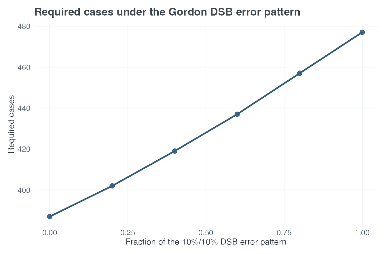
Required case sample size as the Gordon DSB error pattern increases from no error to delta = epsilon = 0.10.

The curve is a design sensitivity analysis: it treats error rates as fixed scenarios rather than estimating their uncertainty.

Published-example reproduction: Edwards et al. (2005)

Edwards et al. examined phenotype error in a biallelic case-control design. Their Figure 2 example uses 250 cases, 250 controls, alpha = 0.01, affected minor-allele frequency 0.05, unaffected minor-allele frequency 0.15, and HWE.

g_edwards_affected <- c(0.9025, 0.0950, 0.0025)
g_edwards_unaffected <- c(0.7225, 0.2550, 0.0225)

edwards_scenarios <- data.frame(
  prev = c(0.05, 0.01, 0.05, 0.01),
  theta = 0,
  phi = c(0.01, 0.01, 0.02, 0.02),
  published_power = c(0.91, 0.33, 0.76, 0.11)
)

edwards_scenarios$paweh_power <- vapply(seq_len(nrow(edwards_scenarios)), function(i) {
  cc_power(
    N_case = 250, alpha = 0.01, k = 1,
    input_mode = "model_free",
    g1 = g_edwards_affected, g0 = g_edwards_unaffected,
    prev = edwards_scenarios$prev[i],
    pheno_misclass = TRUE,
    theta = edwards_scenarios$theta[i],
    phi = edwards_scenarios$phi[i],
    verbose = FALSE
  )$tests$genotypes$power
}, numeric(1))

edwards_scenarios
#>   prev theta  phi published_power paweh_power
#> 1 0.05     0 0.01            0.91   0.9134913
#> 2 0.01     0 0.01            0.33   0.3320457
#> 3 0.05     0 0.02            0.76   0.7633919
#> 4 0.01     0 0.02            0.11   0.1098263

This is an excellent Published-example reproduction; the paper reports rounded powers. Here theta = Pr(affected -> control) and phi = Pr(unaffected -> case). For a rare disease, even a small phi can matter greatly because the unaffected source population is much larger than the affected source population. The no-error reference power is about 0.9896.

Extending Edwards: prevalence and false-positive classification

Both plots use the same underlying genotype distributions. Only prevalence is changed between panels.

plot_cc_power(
  x_var = "phi", x_values = edwards_phi,
  test = "genotypes", input_mode = "model_free",
  N_case = 250, alpha = 0.01, k = 1,
  g1 = g_edwards_affected, g0 = g_edwards_unaffected,
  prev = 0.05, pheno_misclass = TRUE, theta = 0,
  title = "Power vs phenotype misclassification (prevalence 0.05)"
)

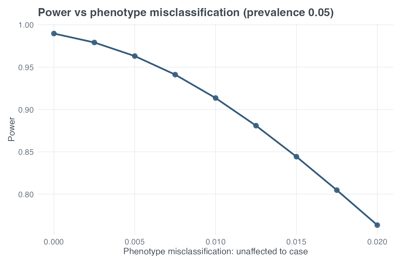
Power as unaffected subjects are increasingly classified as cases, with prevalence 0.05.

plot_cc_power(
  x_var = "phi", x_values = edwards_phi,
  test = "genotypes", input_mode = "model_free",
  N_case = 250, alpha = 0.01, k = 1,
  g1 = g_edwards_affected, g0 = g_edwards_unaffected,
  prev = 0.01, pheno_misclass = TRUE, theta = 0,
  title = "Power vs phenotype misclassification (prevalence 0.01)"
)

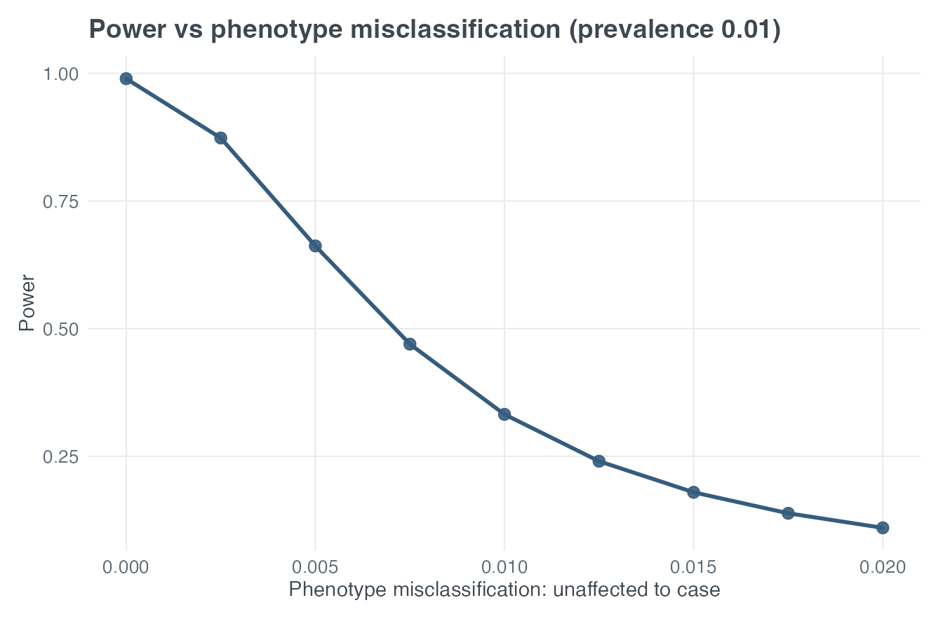
The same sensitivity analysis with prevalence 0.01.

Locus heterogeneity and the trend test

For case-control calculations, pi is the fraction of cases attributable to the modeled locus; 1 - pi is the heterogeneous fraction. The model-free example below compares genotype and trend-test MSSN as heterogeneity grows.

plot_cc_mssn(
  x_var = "locus_het_rate",
  x_values = seq(0, 0.50, by = 0.10),
  input_mode = "model_free", compare_tests = TRUE,
  sample_size = "case",
  power = 0.80, alpha = 0.05, k = 1,
  g1 = g_gordon_case, g0 = g_gordon_control,
  title = "Required cases vs locus heterogeneity"
)

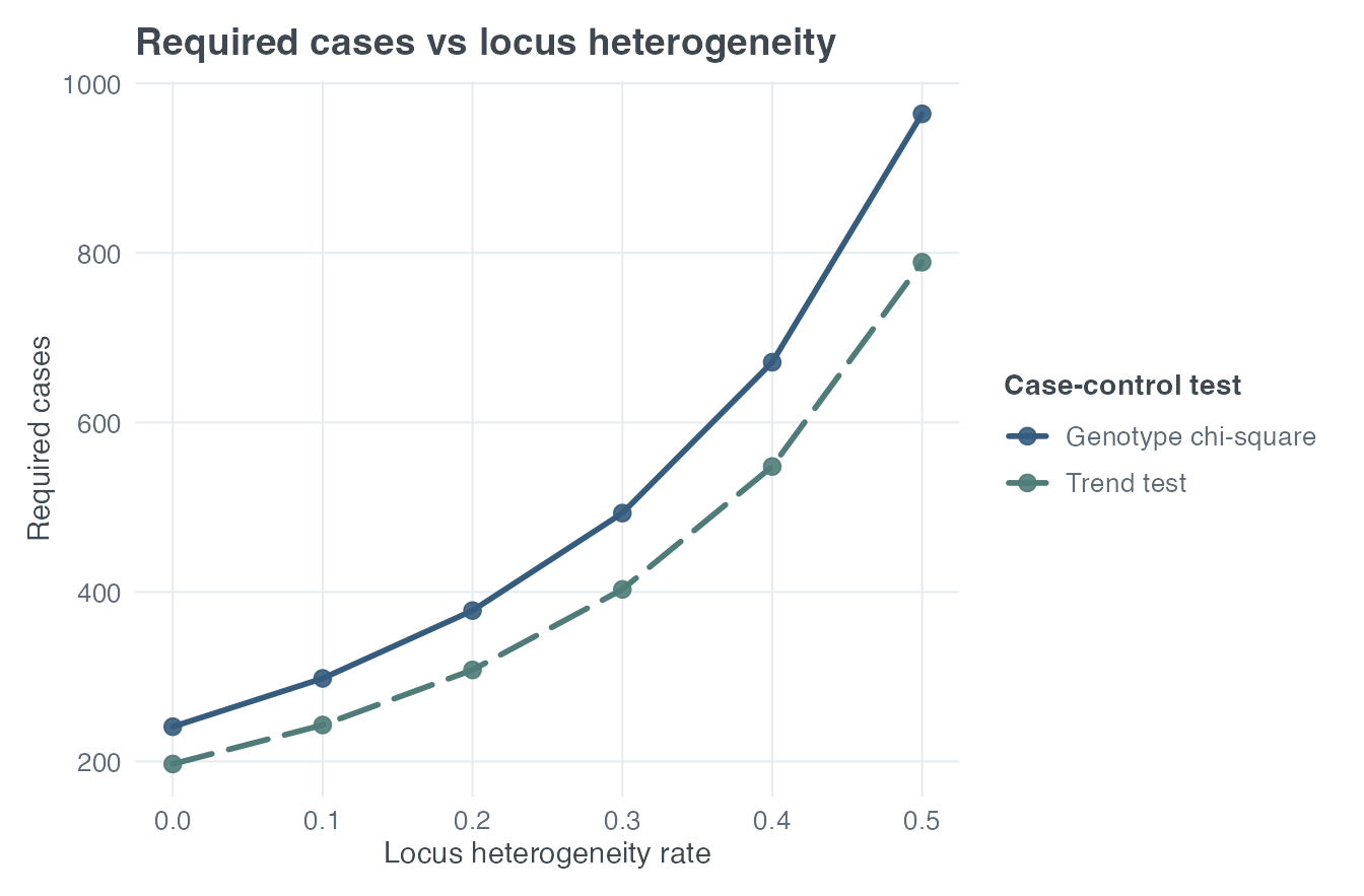
$Required cases for genotype and trend tests as the heterogeneous fraction increases.$

Required cases for genotype and trend tests as the heterogeneous fraction increases.

Ahn et al. (2007) provide Published methodological context for how SNP genotyping errors affect Cochran–Armitage trend-test designs. The plot above does not claim to reproduce their specific Taylor-series error framework.

Differential genotype error: a Type I error warning

Moskvina et al. (2006) showed that different error mechanisms in cases and controls can substantially inflate Type I error, even when absolute error rates are small. The following calculation is therefore context, not a calibrated false-positive analysis.

diff_error_design <- cc_power(
  N_case = 500, alpha = 0.05, k = 1,
  input_mode = "model_free",
  g1 = g_gordon_case, g0 = g_gordon_control,
  geno_misclass = "diff3p",
  case_e01 = 0.02, case_e02 = 0.01, case_e03 = 0.005,
  ctrl_e01 = 0.01, ctrl_e02 = 0.005, ctrl_e03 = 0.002,
  verbose = FALSE
)
diff_error_design$tests$genotypes$power
#> [1] 0.9794989

Important: paweh returns nominal asymptotic power or MSSN under differential genotype error using the usual chi-square critical value. It does not independently recalibrate an arbitrary differential-error null distribution. These nominal operating characteristics must not be interpreted as protection against the Type I error inflation described by Moskvina et al.

Independent sensitivity scenarios

The unified interface accepts several modifiers in one call and reports each as a separate sensitivity scenario from the same no-error baseline. It does not combine the modifier transformations.

scenario_cc <- cc_mssn(
  power = 0.80, alpha = 0.05, k = 1,
  input_mode = "model_free",
  g1 = g_gordon_case, g0 = g_gordon_control,
  locus_het = TRUE, pi = 0.80,
  prev = 0.05, pheno_misclass = TRUE, theta = 0.02, phi = 0.01,
  geno_misclass = "2p", e1 = 0.02, e2 = 0.01,
  verbose = FALSE
)

lapply(scenario_cc$scenarios, function(scenario) {
  c(
    genotype_cases = scenario$tests$genotypes$MSSN_case,
    trend_cases = scenario$tests$trend$MSSN_case
  )
})
#> $no_error
#> genotype_cases    trend_cases 
#>            241            197 
#> 
#> $phenotype_misclassification
#> genotype_cases    trend_cases 
#>            345            282 
#> 
#> $heterogeneity
#> genotype_cases    trend_cases 
#>            378            308 
#> 
#> $genotype_misclassification
#> genotype_cases    trend_cases 
#>            251            205

Choosing an interface and recognizing limits

Use cc_power() and cc_mssn() for most designs, particularly when switching between model-based and model-free inputs or comparing modifier scenarios. Specialized genotype-only functions remain available in the reference manual for focused calculations.

Interpretation depends on assumptions close to each calculation:

HWE was used to construct genotype probabilities in the published examples.
Model-free probabilities are treated as supplied truth, not estimated with uncertainty.
Model-based results inherit the selected prevalence, risk, and inheritance model.
theta and phi describe opposite phenotype-error directions.
pi is the homogeneous fraction; 1 - pi is heterogeneous.
Genotype and trend calculations use asymptotic chi-square approximations.
Integer MSSNs are ceiling values; a paper using another rounding convention can differ by one subject.
Differential genotype error can invalidate nominal Type I error calibration.

References

Ahn K, Haynes C, Kim W, St Fleur R, Gordon D, Finch SJ. The effects of SNP genotyping errors on the power of the Cochran-Armitage linear trend test for case/control association studies. Annals of Human Genetics. 2007;71(Pt 2):249–261. https://doi.org/10.1111/j.1469-1809.2006.00318.x.

Edwards BJ, Haynes C, Levenstien MA, Finch SJ, Gordon D. Power and sample size calculations in the presence of phenotype errors for case/control genetic association studies. BMC Genetics. 2005;6:18. https://doi.org/10.1186/1471-2156-6-18.

Gordon D, Finch SJ, Nothnagel M, Ott J. Power and sample size calculations for case-control genetic association tests when errors are present: application to single nucleotide polymorphisms. Human Heredity. 2002;54(1):22–33. https://doi.org/10.1159/000066696.

Moskvina V, Craddock N, Holmans P, Owen MJ, O’Donovan MC. Effects of differential genotyping error rate on the type I error probability of case-control studies. Human Heredity. 2006;61(1):55–64. https://doi.org/10.1159/000092553.

Session information

sessionInfo()
#> R version 4.6.1 (2026-06-24)
#> Platform: aarch64-apple-darwin23
#> Running under: macOS Tahoe 26.6.2
#> 
#> Matrix products: default
#> BLAS:   /Library/Frameworks/R.framework/Versions/4.6/Resources/lib/libRblas.0.dylib 
#> LAPACK: /Library/Frameworks/R.framework/Versions/4.6/Resources/lib/libRlapack.dylib;  LAPACK version 3.12.1
#> 
#> locale:
#> [1] C.UTF-8/C.UTF-8/C.UTF-8/C/C.UTF-8/C.UTF-8
#> 
#> time zone: America/New_York
#> tzcode source: internal
#> 
#> attached base packages:
#> [1] stats     graphics  grDevices utils     datasets  methods   base     
#> 
#> other attached packages:
#> [1] paweh_0.99.0     BiocStyle_2.40.0
#> 
#> loaded via a namespace (and not attached):
#>  [1] gtable_0.3.6        jsonlite_2.0.0      dplyr_1.2.1        
#>  [4] compiler_4.6.1      BiocManager_1.30.27 tidyselect_1.2.1   
#>  [7] dichromat_2.0-1     jquerylib_0.1.4     systemfonts_1.3.2  
#> [10] scales_1.4.0        textshaping_1.0.5   yaml_2.3.12        
#> [13] fastmap_1.2.0       ggplot2_4.0.3       R6_2.6.1           
#> [16] labeling_0.4.3      generics_0.1.4      knitr_1.51         
#> [19] htmlwidgets_1.6.4   tibble_3.3.1        bookdown_0.47      
#> [22] desc_1.4.3          bslib_0.12.0        pillar_1.11.1      
#> [25] RColorBrewer_1.1-3  rlang_1.3.0         cachem_1.1.0       
#> [28] xfun_0.60           fs_2.1.0            sass_0.4.10        
#> [31] S7_0.2.2            otel_0.2.0          cli_3.6.6          
#> [34] withr_3.0.3         pkgdown_2.2.1       magrittr_2.0.5     
#> [37] digest_0.6.39       grid_4.6.1          mvtnorm_1.4-2      
#> [40] lifecycle_1.0.5     vctrs_0.7.3         evaluate_1.0.5     
#> [43] glue_1.8.1          farver_2.1.2        ragg_1.5.2         
#> [46] rmarkdown_2.31      pkgconfig_2.0.3     tools_4.6.1        
#> [49] htmltools_0.5.9

paweh package authors