Interactive Study Design with the paweh Dashboard

Introduction

paweh includes an interactive Shiny interface for Case-Control, TDT / Family, and Quantitative Trait study-design calculations. The dashboard uses the same canonical statistical functions as the programmatic R interface; it is an interface to those functions, not a separate statistical engine.

This guide focuses on navigating the interface and carrying a design through its workflow. For statistical definitions, assumptions, and derivations, use the study-specific vignettes linked throughout this guide.

Launching the dashboard

Construct the application and then launch the returned object explicitly:

app <- paweh_app()
shiny::runApp(app)

paweh_app() returns a shiny.appobj; it does not launch the application automatically. Keeping construction and launch separate is useful in scripts, tests, and deployment tooling. The vignette does not execute runApp().

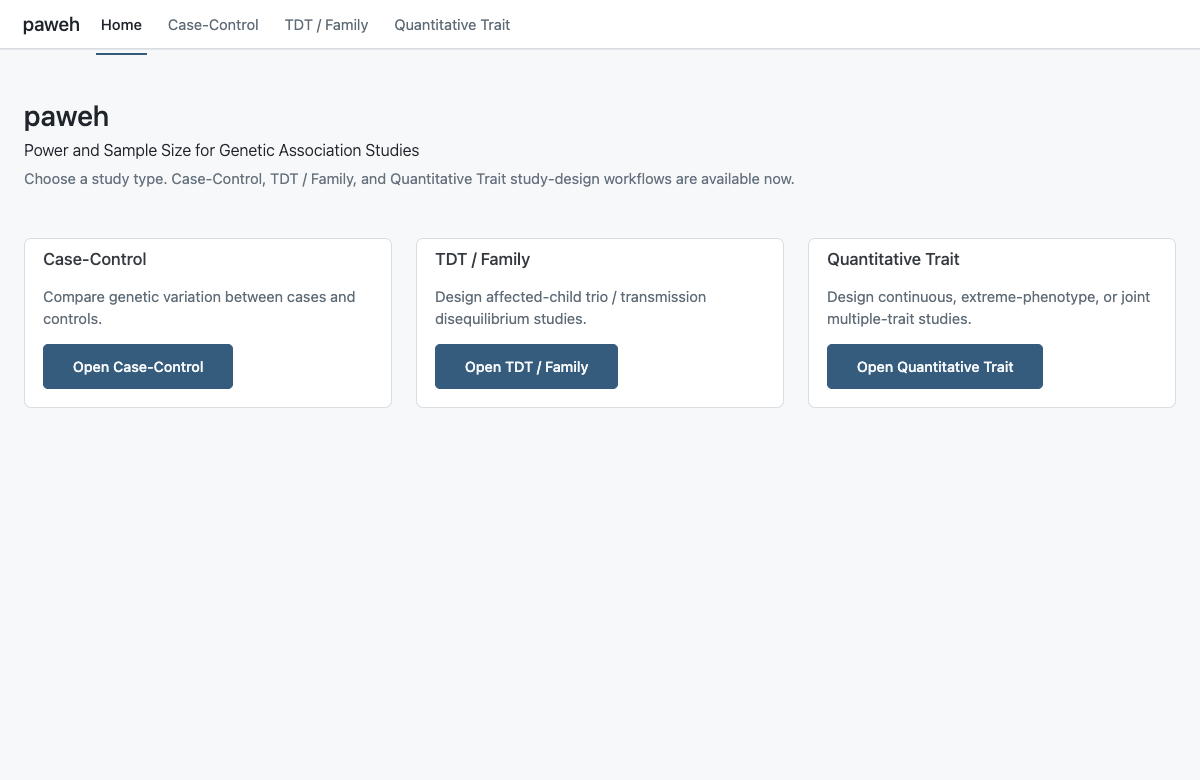
Home page of the paweh dashboard showing Case-Control, TDT or Family, and Quantitative Trait study families.

The paweh dashboard organizes study design by study family, with a dedicated workspace for each supported design.

A typical workflow begins the same way in each workspace:

Choose a study family.
Select Estimate power or Minimum sample size.
Enter the model assumptions.
Select Calculate study design.

The Case-Control and TDT / Family workspaces then provide Results, Sensitivity, Visualize, and Methods tabs, plus advanced details and a reproducible R call. The Quantitative Trait workspace is intentionally simpler: its Output card displays the verbose output from the corresponding canonical QTL function.

Frozen calculated design. Selecting Calculate study design evaluates the current inputs. Editing an input afterward does not partially update the previous result. The Case-Control and TDT / Family workspaces ask the user to recalculate to update their panels; the Quantitative Trait workspace reports “Inputs have changed. Recalculate to update output.”

Case-Control workflow

The Case-Control workspace compares genotype distributions between cases and controls. Choose whether to estimate power at a specified number of cases or find the minimum sample size for a target power. Inputs may be specified as a genetic model or as direct case and control genotype probabilities.

For a model-based design, core assumptions include disease prevalence, modeled-allele frequency, the homozygote relative risk and mode of inheritance, the case-to-control allocation, and the significance level. Advanced options cover phenotype misclassification, genotype misclassification, and locus heterogeneity. Their statistical definitions are described in the Case-Control Study Design vignette.

A representative programmatic calculation corresponding to the dashboard is:

cc_design <- cc_power(
  N_case = 500,
  alpha = 0.05,
  input_mode = "model_based",
  prev = 0.10,
  pd = 0.30,
  R2 = 2,
  MOI = "M",
  k = 1,
  verbose = FALSE
)

data.frame(
  test = c("Genotype chi-square", "Trend"),
  power = c(cc_design$tests$genotypes$power, cc_design$tests$trend$power)
)
#>                  test     power
#> 1 Genotype chi-square 0.9619099
#> 2               Trend 0.9821860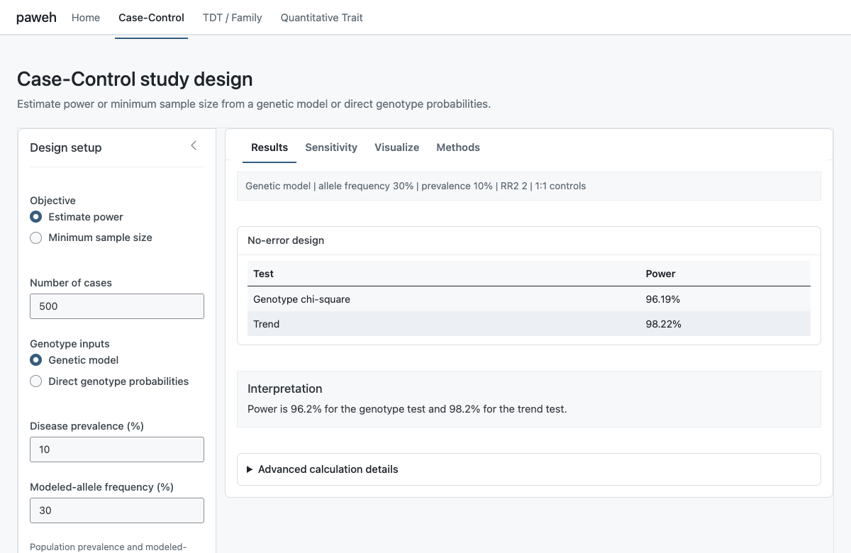

Case-Control dashboard showing calculated genotype chi-square and trend-test power with the frozen study-design summary.

The Case-Control Results tab summarizes genotype chi-square and trend-test power for the frozen study design, with advanced calculation details available for review.

For power, Results reports the expected power of the genotype chi-square and trend tests. For minimum sample size, it reports the required design size. When an effective modifier is active, the dashboard distinguishes the no-error baseline from adjusted results. These are deterministic calculations under the entered assumptions, not estimates from observed data.

In Sensitivity, select one parameter and a range. Every other assumption stays at its frozen value, and a vertical marker identifies the calculated design. The plot may use a tightly zoomed y-axis to make small changes in power visible; the interface notes when it does so. Visualize presents the current case-control genotype comparison using the frozen design.

TDT / Family workflow

The TDT / Family workspace designs transmission disequilibrium studies in affected-child trios; the trio, rather than an individual participant, is the sampling unit. Choose power or minimum sample size, then specify either a genetic model or direct expected transmission quantities. Model-based inputs include the heterozygote relative risk (R1), homozygote relative risk (R2), and linkage disequilibrium measure D-prime, along with prevalence and allele frequency. See TDT Study Design for the underlying statistical model.

Separate TDT modifier scenarios. Phenotype misclassification and locus heterogeneity are evaluated as separate TDT sensitivity scenarios. When both are enabled, the dashboard displays (1) the baseline/no-error design, (2) the phenotype-misclassification scenario, and (3) the locus-heterogeneity scenario. It does not interpret them as one joint combined TDT model.

For a genetic-model input, Advanced assumptions also offers the exact control Genotype misclassification (Chapter 5). Selecting it reveals Genotype misclassification rate (%), which accepts a percentage from 0 to 50; the interface converts that value to the package-scale proportion supplied as genotype_misclassification_rate. This model is unavailable for direct transmission quantities and must be used separately from phenotype misclassification and locus heterogeneity. The interface reports a clear error if those constraints are violated.

The Results and advanced-details panels report the no-error and Chapter 5 genotype-misclassification quantities returned by tdt_power() or tdt_mssn(), including retained and Mendelian-inconsistent trio probabilities. Sensitivity and advanced surface plots are not provided for this genotype-error branch.

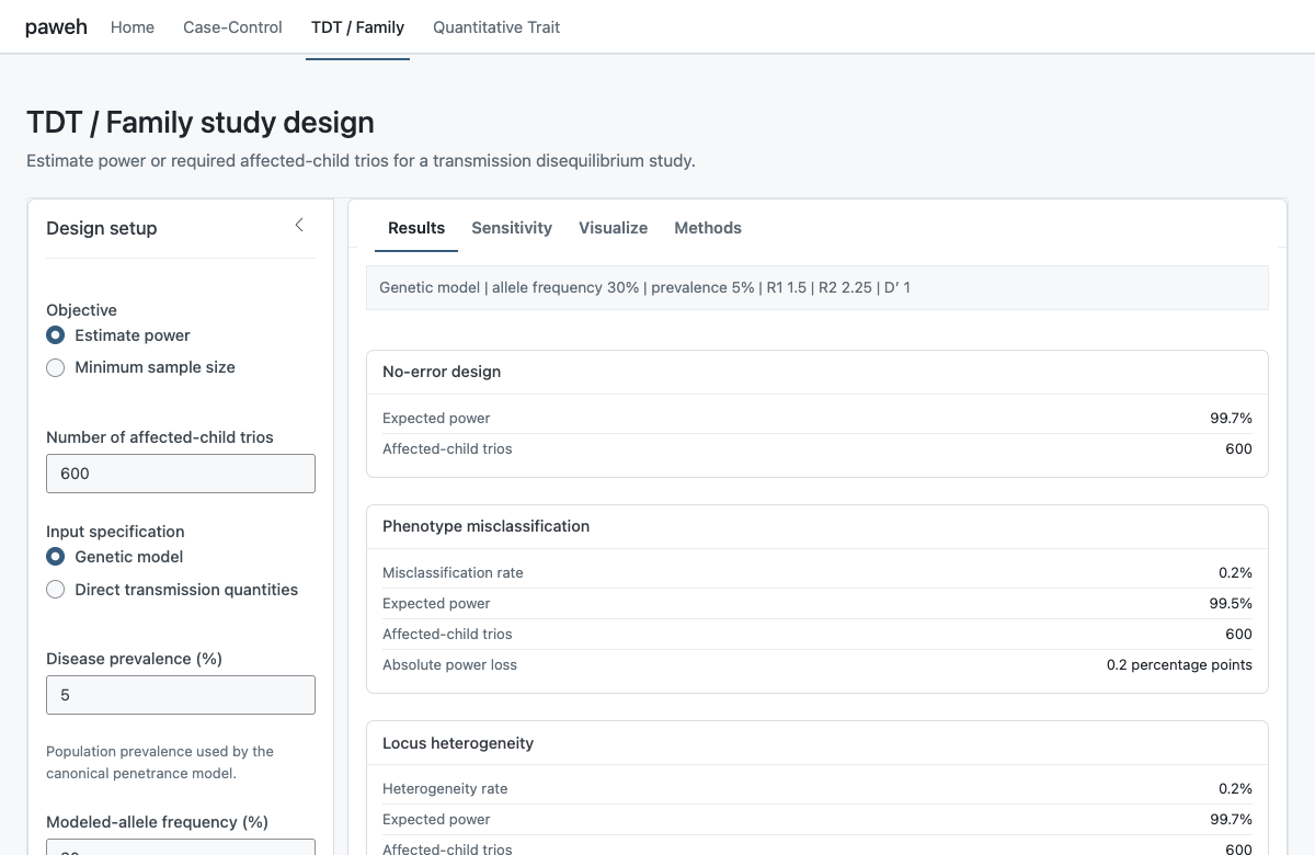
TDT dashboard displaying baseline, phenotype-misclassification, and locus-heterogeneity power scenarios separately.

The TDT Results tab keeps the baseline, phenotype-misclassification, and locus-heterogeneity scenarios separate when both modifiers are requested.

The transmission visualization compares expected transmitted and non-transmitted quantities and labels them numerically from the canonical TDT result. Sensitivity varies one parameter at a time while preserving the other frozen assumptions.

An optional 3D surface explores two assumptions simultaneously. It is generated only after the user requests it, uses the frozen model-based design, and does not alter the primary calculation. Rotate the Plotly surface with click and drag, and zoom or inspect values interactively.

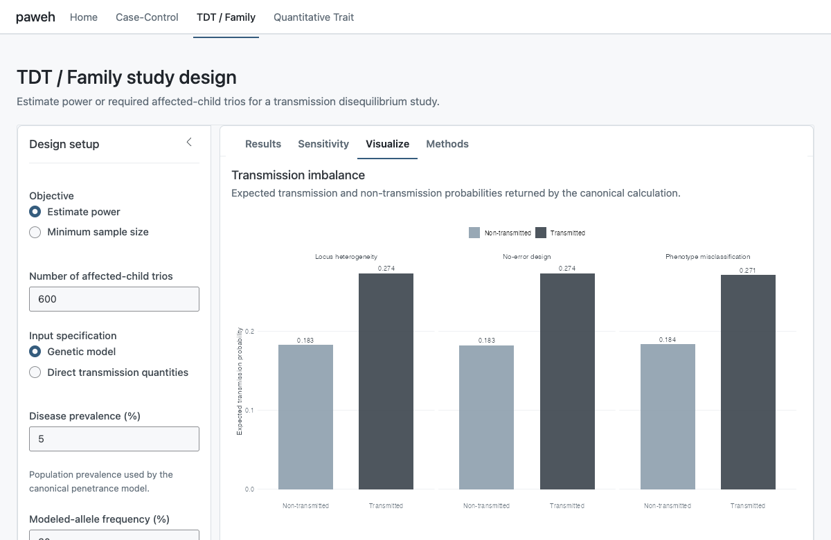
Three-dimensional TDT power surface over allele frequency and phenotype-misclassification rate.

The optional TDT 3D surface explores two assumptions simultaneously while retaining the last calculated model-based design.

Quantitative Trait workflow

The Quantitative Trait workspace is a thin input interface over the public QTL functions. Its workflow is deliberately direct:

$\text{inputs} \longrightarrow \text{Calculate study design} \longrightarrow \text{canonical verbose PAWEH output}.$

Choose Estimate power or Minimum sample size, enter the model inputs, and select Calculate study design. The single Output card then shows the verbose console presentation generated by the corresponding canonical function. There are no QTL Results, Sensitivity, Visualize, Methods, advanced decomposition, or 2-D/3-D Plotly panels in the current dashboard.

The workspace exposes three designs:

Full continuous trait calls qtl_anova_power() or qtl_anova_mssn().
Extreme phenotype sampling calls qtl_threshold_chisq_power() or qtl_threshold_chisq_mssn().
Multiple quantitative traits calls qtl_multivariate_power_full() or qtl_multivariate_mssn_full(), using either the Pillai continuous-trait test or joint threshold-selected genotype chi-square test.

Common controls include objective-specific sample size or target power, significance level, and modeled-allele frequency. The continuous design adds QTL variance, dominance, and genotype-count options. The extreme design adds upper- and lower-tail percentages and their selected-sample ratio. The multivariate design accepts two to four phenotype-specific QTL variances and dominance values, pairwise phenotype correlations, and joint-tail inputs when the threshold test is selected.

If inputs change after a calculation, the previous verbose output remains visible with the notice Inputs have changed. Recalculate to update output. The Quantitative-Trait Study Design vignette provides the statistical interpretation and approved model visualizations outside the dashboard.

Full continuous trait

This design analyzes the measured quantitative phenotype directly. Enter total sample size for power or target power for MSSN, QTL variance explained, dominance, allele frequency, and the optional genotype-count settings. The Output card presents the canonical ANOVA result.

Extreme phenotype sampling

This design analyzes individuals selected from the lower and upper phenotype tails. The user enters population-tail percentages and an upper-tail selected sample for power, or target power for MSSN. The model determines the phenotype thresholds, and the Output card reports the canonical threshold-design result.

Multiple quantitative traits

The calculation supports two to four traits, with trait-specific variance explained and dominance values plus pairwise phenotype correlations. Choose a Pillai continuous-trait test or joint extreme-selection test. For the latter, enter upper and lower percentages for every trait and the lower-to-upper selected-sample ratio. All selected traits enter the canonical calculation; the current QTL workspace does not add a separate plot.

Detailed panels in Case-Control and TDT

In the Case-Control and TDT / Family workspaces, Advanced calculation details exposes deeper quantities returned by the same canonical calculation used for the primary result. Depending on the workflow, these can include genotype probabilities, expected transmission quantities, noncentrality parameters, degrees of freedom, and fractional minimum sample size. Not every field appears for every model.

Methods summarizes the statistical procedure and assumptions for the frozen design. It complements Advanced calculation details: Methods explains what procedure is being used, while Advanced calculation details shows quantities produced by that calculation. These panels are not part of the current Quantitative Trait workspace.

Reproduce calculations in R

The Case-Control and TDT / Family advanced details include a Reproduce in R block generated from the frozen inputs. It uses the same canonical public function and arguments as the dashboard calculation. For example, a model-based TDT design may produce:

tdt_power(
  N = 600,
  alpha = 0.05,
  input_mode = "model_based",
  prev = 0.05,
  pd = 0.30,
  R1 = 1.5,
  R2 = 2.25,
  delta_prime = 1,
  verbose = FALSE
)

Copy this code into a script to preserve or extend the design. For QTL, use the canonical function identified above with the same inputs entered in the GUI; the dashboard itself displays that function’s verbose output rather than a separate generated call block.

Frequently asked questions

Why did my result not change when I edited an input?

The dashboard preserves the last calculated design until Calculate study design is selected again.

Why is the sensitivity plot y-axis zoomed?

A tighter scale makes small changes in power easier to see. The dashboard displays a note when the scale is tightly zoomed.

Why can minimum sample size be Inf?

For a model with no detectable contrast or effect, no finite sample size can reach the requested power.

Why are TDT error and heterogeneity mechanisms shown separately?

Phenotype misclassification and locus heterogeneity are separate sensitivity scenarios rather than one combined model. Chapter 5 genotype misclassification is also modeled separately and cannot be combined with either of them.

Why does the QTL workspace show only console-style output?

It is intentionally a thin GUI over the canonical QTL functions. The dedicated QTL vignette and plotting functions provide model visualizations.

Why does the TDT 3D plot not appear immediately?

The TDT Plotly surface is generated on demand to keep startup responsive.

What is the difference between Advanced calculation details and Methods in the Case-Control and TDT workspaces?

Advanced details shows model and calculation quantities; Methods summarizes the statistical procedure and assumptions.

Dashboard and programmatic workflows

Use the Case-Control and TDT / Family workspaces for interactive study planning, sensitivity inspection, and visualization. Use the Quantitative Trait workspace as a compact input front end to canonical verbose output. Use the public R functions for scripted workflows, reproducible pipelines, batch analyses, and code accompanying manuscripts or supplements. Every workspace delegates its calculations to the same statistical backend as those functions.

Session information

sessionInfo()
#> R version 4.6.1 (2026-06-24)
#> Platform: aarch64-apple-darwin23
#> Running under: macOS Tahoe 26.6.2
#> 
#> Matrix products: default
#> BLAS:   /Library/Frameworks/R.framework/Versions/4.6/Resources/lib/libRblas.0.dylib 
#> LAPACK: /Library/Frameworks/R.framework/Versions/4.6/Resources/lib/libRlapack.dylib;  LAPACK version 3.12.1
#> 
#> locale:
#> [1] C.UTF-8/C.UTF-8/C.UTF-8/C/C.UTF-8/C.UTF-8
#> 
#> time zone: America/New_York
#> tzcode source: internal
#> 
#> attached base packages:
#> [1] stats     graphics  grDevices utils     datasets  methods   base     
#> 
#> other attached packages:
#> [1] paweh_0.99.0     BiocStyle_2.40.0
#> 
#> loaded via a namespace (and not attached):
#>  [1] gtable_0.3.6        jsonlite_2.0.0      dplyr_1.2.1        
#>  [4] compiler_4.6.1      BiocManager_1.30.27 tidyselect_1.2.1   
#>  [7] dichromat_2.0-1     jquerylib_0.1.4     systemfonts_1.3.2  
#> [10] scales_1.4.0        textshaping_1.0.5   yaml_2.3.12        
#> [13] fastmap_1.2.0       ggplot2_4.0.3       R6_2.6.1           
#> [16] generics_0.1.4      knitr_1.51          htmlwidgets_1.6.4  
#> [19] tibble_3.3.1        bookdown_0.47       desc_1.4.3         
#> [22] bslib_0.12.0        pillar_1.11.1       RColorBrewer_1.1-3 
#> [25] rlang_1.3.0         cachem_1.1.0        xfun_0.60          
#> [28] fs_2.1.0            sass_0.4.10         S7_0.2.2           
#> [31] otel_0.2.0          cli_3.6.6           pkgdown_2.2.1      
#> [34] magrittr_2.0.5      digest_0.6.39       grid_4.6.1         
#> [37] mvtnorm_1.4-2       lifecycle_1.0.5     vctrs_0.7.3        
#> [40] evaluate_1.0.5      glue_1.8.1          farver_2.1.2       
#> [43] ragg_1.5.2          rmarkdown_2.31      pkgconfig_2.0.3    
#> [46] tools_4.6.1         htmltools_0.5.9

paweh package authors